
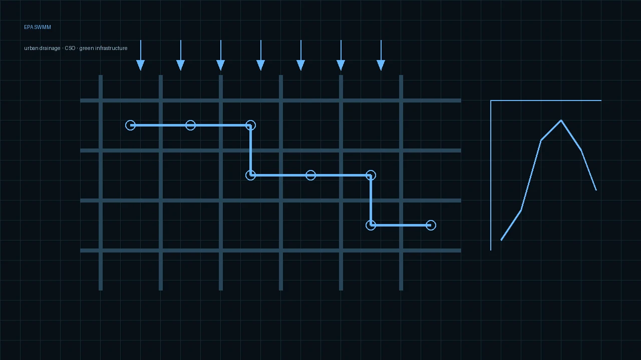
When we think of floods we usually imagine a river overflowing.
But in a city the problem can be completely different.
It can rain intensely without a large river nearby and still produce a flood.
Why?
Because the city changes the water cycle.
natural soil
↓
infiltration

city
↓
roof + pavement + streets
↓
fast runoff
↓
inlets
↓
pipes
↓
overload
↓
flooding
EPA SWMM was born to understand this kind of urban system.
And its history begins in 1971, barely a year after the creation of the U.S. Environmental Protection Agency.
The United States and the urban pollution problem
During the 1960s and 1970s the United States faced enormous problems of water-body pollution.
A particularly important problem was Combined Sewer Overflows — CSO.
In older cities, the same system could carry:
wastewater
+
stormwater
During a storm, the system could exceed its capacity.
Then a contaminated mixture ended up discharging directly into rivers.
It was necessary to understand:
- how much runoff the city produced;
- how it moved through the network;
- when the system overloaded;
- which pollutants it carried.
1971: SWMM is born
EPA records 1971 as the year of development and release of the first version of the Storm Water Management Model — SWMM.
The initial development involved:
- Metcalf & Eddy;
- Water Resources Engineers;
- University of Florida;
with funding from the federal agency.
The first version was written in FORTRAN.
The original SWMM was not simply a hydraulic model
From the beginning the goal combined:
hydrology
+
hydraulics
+
water quality
That remains a central feature of the program.
SWMM can model:
- precipitation;
- infiltration;
- runoff;
- pipes;
- channels;
- storage;
- pumps;
- regulators;
- pollutants.
SWMM I
The first generation was aimed especially at problems of:
- CSO;
- urban runoff;
- pollution.
Compared with the modern program it was limited.
But the conceptual architecture was already appearing.
A city could be divided into subcatchments that produce runoff.
That runoff enters a drainage system.
And then it is routed through the network.
1975: SWMM II
In 1975, the University of Florida produced a version that became the first widely distributed one.
SWMM was beginning to consolidate.
1981: SWMM 3
In 1981, SWMM 3 introduced important advances.
Among them:
- dynamic wave flow;
- Green-Ampt infiltration;
- snowmelt;
- continuous simulation.
That transformed the physical capability of the model in a significant way.
Dynamic Wave
Hydraulic routing can be approximated at different levels of complexity.
At the most complete extreme we find dynamic wave formulations.
These use the complete Saint-Venant equations for 1D flow.
Conceptually:
conservation of mass
+
conservation of momentum
This can represent phenomena such as:
- surcharge;
- backwater;
- reversals;
- complex networks.
1983: SWMM reaches the PC
Version SWMM 3.3, in 1983, was the first version for personal computers.
This was hugely important.
Just as AutoCAD democratized CAD through the PC, SWMM began to bring urban hydrologic-hydraulic simulation closer to more engineers.
1988: SWMM 4
In 1988 SWMM 4 appears.
Institutions such as these took part:
- Oregon State University;
- Camp Dresser & McKee.
SWMM 4 added and refined capabilities such as:
- groundwater;
- RDII;
- irregular sections;
- hydraulic improvements.
During the 1990s it continued to evolve.
PCSWMM and the commercial ecosystem
While EPA developed SWMM, other organizations built interfaces and tools around the engine.
One of the best known is PCSWMM.
This shows something important about SWMM:
the engine ended up becoming a kind of de facto standard on which specialized software could be built.
2002: a radical decision
In the early 2000s EPA decided to modernize the program completely.
They did not want simply to add another layer of patches on top of SWMM 4.
In 2002 an agreement was established between EPA and CDM-Smith to rewrite the model.
The result would be SWMM 5.
2005: SWMM 5
In 2005 SWMM 5 was published.
It was an enormous transformation.
The engine was completely rewritten in C.
A modern graphical interface was also incorporated.
That created the base of the SWMM we still know.
The modern conceptual model
SWMM divides the system into different components.
Subcatchments
They represent zones that receive precipitation.
rain
↓
subcatchment
↓
runoff
Nodes
They can represent:
- junctions;
- storage;
- outfalls;
- dividers.
Links
They can be:
- conduits;
- pumps;
- orifices;
- weirs;
- outlets.
What is SWMM used for?
1. Storm drainage
The best-known use.
It can represent:
subcatchment
↓
inlet
↓
pipe
↓
collector
↓
outfall
And calculate:
- discharge;
- depth;
- surcharge;
- flooding.
2. Combined sewers
This was one of its original problems.
It can study when a mixed network exceeds its capacity and discharges.
3. Sanitary sewers
It can also represent sanitary systems and processes such as RDII — Rainfall-Derived Infiltration and Inflow.
This helps study how rain and groundwater introduce parasitic water into the sanitary system.
4. Urban flooding
SWMM can identify nodes where the system exceeds its capacity.
The standard version is fundamentally a 1D network model.
To represent in detail how water moves over streets and terrain it can be integrated with other 2D models or specialized tools.
5. Long-Term Continuous Simulation
It is not limited to a single storm.
It can simulate:
months
years
including moisture and infiltration cycles.
This is especially useful for evaluating the performance of green infrastructure.
Infiltration
SWMM has several methods to represent infiltration.
Among them:
- Horton;
- Green-Ampt;
- Curve Number.
The choice directly affects how much runoff is generated.
LID: Low Impact Development
One of the most important evolutions was the incorporation of LID Controls.
They can represent strategies such as:
- bioretention;
- rain gardens;
- permeable pavement;
- green roofs;
- infiltration trenches;
- rain barrels;
- vegetative swales.
Conceptually:
rain
↓
green infrastructure
↓
storage / infiltration
↓
less runoff
This moved SWMM from the classical logic of:
get the water out as fast as possible
toward:
manage the water where it falls.
Water quality
SWMM can also represent:
- pollutant buildup;
- washoff;
- transport;
- treatment.
This reflects its historical origin in pollution control.
The system does not only answer:
how much water?it can also study:
what does that water carry?Controls
SWMM can represent operating rules.
For example:
if tank level > X
→ turn pump on

if level < Y
→ turn pump off
This makes it possible to simulate networks with dynamic operation.
Streets and inlets
Generation 5.2 incorporated important capabilities to represent:
- streets;
- inlet capture;
using methodologies such as FHWA HEC-22.
This is especially interesting for urban drainage because it can better represent the connection between:
surface runoff
↓
street
↓
inlet
↓
underground network
SWMM vs HEC-HMS
Both can model rainfall-runoff.
But their specialization is different.
HEC-HMS
Very strong in:
- watersheds;
- hydrology;
- channel routing;
- reservoirs;
- hydrographs.
SWMM
Very strong in:
- the city;
- pipes;
- sewer networks;
- inlets;
- pumps;
- storage;
- water quality;
- LID.
A large rural watershed:
HEC-HMSA detailed urban drainage network:
SWMMusually makes more sense.
SWMM vs HEC-RAS
SWMM
Represents very well:
drainage networkHEC-RAS
Represents very well:
rivers
+
floodplains
+
1D/2D flow
In a complex urban flood there can be hybrid workflows or commercial tools that combine a 1D network and a 2D surface.
SWMM vs EPANET
Both have a historical relationship with EPA.
But they solve different networks.
EPANET
drinking water
+
pressurized network
SWMM
stormwater / sewer
+
free-surface / pressurized conditions
Open software
EPA distributes SWMM as software that is:
- free;
- open;
- with source code publicly available.
The engine is written in C.
This makes it especially attractive for:
- research;
- integrations;
- in-house tools;
- automation.
SWMM Toolkit
Just like EPANET, SWMM can be used as an engine from other applications.
Conceptually:
Python / C / application
↓
SWMM engine
↓
simulation
↓
results
This has created an enormous ecosystem.
Python
There are community libraries and wrappers that can integrate SWMM with Python.
That allows:
- generating models;
- running scenarios;
- calibrating;
- optimizing;
- processing results.
A modern workflow can be:
GIS
↓
create network
↓
SWMM
↓
Python
↓
optimization
↓
dashboard
SWMM and agents
For an AEC harness this is very interesting.
An agent could:
read GIS
↓
create subcatchments
↓
define event
↓
run SWMM
↓
detect flooding
↓
propose alternatives
↓
test LID
↓
compare results
But there must be technical control over:
- infiltration;
- roughness;
- curves;
- boundary conditions;
- calibration.
Current state in 2026
EPA’s official repository continues to maintain the SWMM 5.2 generation.
The most recent official solver release is SWMM 5.2.4, published as an August 2023 build.
EPA continues to present SWMM as open-source, freely accessible software for:
- stormwater;
- combined sewers;
- sanitary sewers;
- green infrastructure.
That a tool from 1971 is still actively used more than fifty years later is extraordinary.
Timeline in brief
1971
SWMM I
FORTRAN
CSO / urban runoff
        ↓
1975
SWMM II
        ↓
1981
SWMM 3
dynamic wave
Green-Ampt
continuous simulation
        ↓
1983
SWMM 3.3
first PC version
        ↓
1988
SWMM 4
        ↓
1990s
ecosystem / PCSWMM
        ↓
2002
rewrite project
        ↓
2005
SWMM 5
engine completely rewritten in C
        ↓
LID
water quality
green infrastructure
        ↓
2022
SWMM 5.2
street/inlet modeling
        ↓
2023–2026
SWMM 5.2.4
Conclusion
SWMM was born to help solve one of the great urban problems of the 1970s:
the pollution produced by drainage and sewer systems during storms.
But it survived because the problem evolved.
Today we need to design cities able to manage:
- intense storms;
- urbanization;
- old infrastructure;
- climate change;
- pollution;
- green infrastructure.
SWMM went from punch cards, FORTRAN, and combined sewer overflows to becoming an open engine able to represent an entire urban stormwater system.
And its greatest strength is probably precisely that:
combine hydrology, hydraulics, operation, and water quality inside the same urban model.
References
- U.S. EPA. Storm Water Management Model (SWMM).
- U.S. EPA. Safe Water Resources Research Milestones.
- U.S. EPA. Storm Water Management Model Reference Manual.
- U.S. EPA. Official SWMM Source Code Repository.
- U.S. EPA. SWMM 5.2 Features.
Evaluation and limitations
Treat the notes below as evaluation context, not as a verified calculation or code check.
Use it for urban drainage, sewers, CSO, water quality, and LID. A large rural watershed is usually HEC-HMS territory; a river and its floodplain, HEC-RAS; a pressurized drinking-water network, EPANET.